Module 04 of 17
Teaching Models New Behaviors
A practitioner's guide to fine-tuning LLMs — when to fine-tune vs RAG vs prompt, how LoRA and QLoRA work without the math, data preparation checklists, cost comparisons, and the OpenAI and HuggingFace workflows.
01. Fine-Tuning vs Prompting — When to Use Which
The most important thing to understand about fine-tuning is that it is not the first tool you should reach for. A large fraction of developers who decide they need to fine-tune have not yet exhausted simpler options. Prompt engineering is free, fast to iterate on, and reversible. RAG injects facts dynamically without training cost. Fine-tuning requires compute, engineering time for data preparation, and produces a static artifact that cannot be easily updated.
The diagnostic question is: is this a knowledge problem or a behavior problem? A knowledge problem means the model does not know certain facts — your internal database, product catalog, or latest regulations. Knowledge problems are almost always better solved by RAG, which injects facts at query time. The model already knows how to reason; you just supply the data.
A behavior problem means the model knows the information but does not act the way you want — wrong tone, wrong format, missing domain conventions, unnecessary caveats. Behavior problems are where fine-tuning shines. It "bakes in" the desired behavior at the weight level, so it persists regardless of what the user says.
Think of it like this: RAG is giving a smart employee a reference manual to consult while working. Fine-tuning is sending that employee to a specialized training program that changes how they approach the work. Both are useful, but you would not send someone to a training program when what they need is a better reference manual.
What This Means for Practitioners: The Decision Framework
| Approach | When to Use | Cost Profile | Best For |
|---|---|---|---|
| Prompt Engineering | Default starting point — behavior already possible, just needs direction | Near zero | Format guidance, tone, persona |
| RAG | Knowledge gap; facts change frequently; need citations | Low (retrieval infrastructure) | Dynamic facts, product catalogs, regulations |
| Fine-Tuning | Persistent behavior change; format consistency; domain vocabulary; cost at scale | High upfront, low per-call | Tone, style, specialized output formats |
| All Three Combined | Production systems at scale | Highest upfront | Maximum quality and efficiency |
Specific scenarios where fine-tuning wins:
- Consistent output format. If your application requires structured JSON with specific fields, a fine-tuned model just produces it without needing format instructions in every call — saving tokens on every request.
- Specialized vocabulary. Medical, legal, and financial domains have terminology so precise that base models make subtle errors. Fine-tuning on domain examples fixes this.
- Latency and cost at scale. A fine-tuned 7B model can match a prompted GPT-4 on a narrow task at 10-100x lower cost and dramatically lower latency. At millions of daily calls, this arithmetic matters enormously.
When NOT to fine-tune:
- Prompt engineering achieves 85-90% of your goal — the remaining gap rarely justifies the cost.
- Your data distribution changes frequently — fine-tuned models are frozen to their training distribution.
- You have fewer than 100 high-quality examples — you will overfit.
Rule of Thumb: Start with prompt engineering. If you hit a ceiling, try RAG. If you still have a behavior problem, then fine-tune. The three approaches are not mutually exclusive.
02. LoRA — How It Works and When to Use It
Before LoRA, fine-tuning a 7B model required updating all 7 billion parameters — 60-80 GB of VRAM for gradients and optimizer states, meaning a cluster of expensive GPUs. LoRA (Low-Rank Adaptation) changed this by introducing small additional matrices alongside the existing weights and only training those. The original weights are frozen and never change.
The key insight is that the meaningful updates during fine-tuning have a much simpler structure than the full weight matrices. Even though a weight matrix might be 4096x4096, the actual changes can be captured by two much smaller matrices multiplied together. A LoRA adapter for a 7B model might be 50-200 MB — less than 2% of the model size.
This has a beautiful practical consequence: you can maintain one base model and a library of many LoRA adapters for different tasks. Need a customer service assistant? Swap in the customer service LoRA. Need a code reviewer? Swap in the code review LoRA. One model, many specialists.
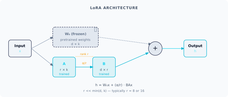
LoRA architecture: the frozen pretrained weight W0 (gray, dashed) passes the input through unchanged, while the trained low-rank matrices A and B (cyan) add a small adaptation. Only A and B are updated during training.
What This Means for Practitioners: LoRA Configuration
The key hyperparameters and what they control:
| Parameter | What It Does | Typical Values | Guidance |
|---|---|---|---|
| rank (r) | Dimensionality of the adapter matrices — higher = more expressive | 4, 8, 16, 32, 64 | Start with r=16. Higher is not always better — low rank is fine for simple behavioral changes |
| alpha | Scaling factor for the LoRA contribution | Often set to 2x rank | Controls how much the adapter affects output. Higher alpha = stronger effect |
| target_modules | Which layers get LoRA adapters | All linear layers | Modern defaults apply to all linear layers, not just q_proj/v_proj |
| dropout | Regularization to prevent overfitting | 0.05 - 0.1 | Increase if you see overfitting with small datasets |
Memory comparison — why LoRA is transformative:
| Method | 7B Model VRAM | 70B Model VRAM | Hardware Needed |
|---|---|---|---|
| Full fine-tuning | ~60 GB | ~600 GB | Multi-GPU cluster |
| LoRA | ~16-18 GB | ~160 GB | Single A100 or RTX 4090 |
| QLoRA (4-bit) | ~6 GB | ~35 GB | Single RTX 3060 or A100 |
At inference time, you have two options: Merge the adapter into the base model (zero latency overhead — just a normal model) or keep them separate for hot-swapping between adapters without reloading the base model.
from peft import LoraConfig, get_peft_model, TaskType

lora_config = LoraConfig(
    task_type=TaskType.CAUSAL_LM,
    r=16,
    lora_alpha=32,
    target_modules=[
        "q_proj", "v_proj", "k_proj", "o_proj",
        "gate_proj", "up_proj", "down_proj"
    ],
    lora_dropout=0.05,
    bias="none",
)

model = get_peft_model(base_model, lora_config)
model.print_trainable_parameters()
# trainable params: 41,943,040 || all params: 7,284,015,104 || trainable%: 0.5757
03. QLoRA — Fine-Tuning Models That Do Not Fit in Memory
QLoRA combines LoRA with 4-bit quantization: compress the base model weights to 4 bits per value, reducing memory by 4x, then apply LoRA on top. The base model is stored in 4-bit but computation happens in 16-bit — weights are dequantized on-the-fly during the forward pass, so gradients flow normally through the LoRA parameters.
This is what made it possible to fine-tune a 70B model on a single GPU. Before QLoRA, that required ~140 GB VRAM (two A100s minimum). With QLoRA, the 70B model fits in ~35 GB — a single A100.
Think of it like this: QLoRA is like compressing a massive reference library into a Kindle. The books are stored in compressed form (4-bit), but when you actually read a page (forward pass), it decompresses to full quality (16-bit). You can only write notes in the margins (LoRA adapters), not change the original text.
What This Means for Practitioners: QLoRA Setup
QLoRA is ~20-30% slower than pure LoRA because of the dequantization overhead. Use LoRA when VRAM allows; use QLoRA when the model would not fit otherwise.
import torch
from transformers import AutoModelForCausalLM, BitsAndBytesConfig
from peft import LoraConfig, get_peft_model, prepare_model_for_kbit_training

bnb_config = BitsAndBytesConfig(
    load_in_4bit=True,
    bnb_4bit_quant_type="nf4",
    bnb_4bit_compute_dtype=torch.bfloat16,
    bnb_4bit_use_double_quant=True,
)

model = AutoModelForCausalLM.from_pretrained(
    "meta-llama/Llama-3.1-8B-Instruct",
    quantization_config=bnb_config,
    device_map="auto",
)
model = prepare_model_for_kbit_training(model)

lora_config = LoraConfig(
    r=16, lora_alpha=32,
    target_modules=["q_proj", "v_proj", "k_proj", "o_proj"],
    lora_dropout=0.05, bias="none", task_type="CAUSAL_LM",
)
model = get_peft_model(model, lora_config)
model.print_trainable_parameters()
# trainable params: 20,971,520 || all params: 8,051,249,152 || trainable%: 0.2604
04. Alignment — RLHF and DPO
After fine-tuning a model to follow instructions (SFT), you can further align it with human preferences. This is what makes ChatGPT feel helpful rather than producing raw text completions.
RLHF (Reinforcement Learning from Human Feedback) works in three stages: (1) SFT to create a baseline assistant, (2) train a reward model on human preference rankings, (3) use PPO to optimize the model against the reward model. It is effective but complex — three separate models, finicky hyperparameters, and 3-10x the compute cost of SFT.
DPO (Direct Preference Optimization) achieves the same goal in a single training step. Instead of training a separate reward model, DPO directly optimizes on preference pairs — (prompt, chosen response, rejected response) triplets. DPO is now the dominant alignment technique for open-weight models. Nearly all fine-tuned open-source models since mid-2023 use DPO rather than RLHF.
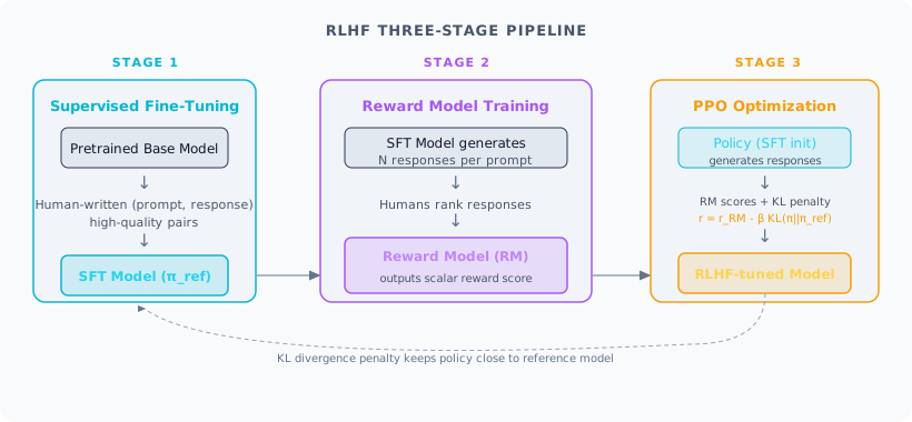
RLHF three-stage pipeline: SFT creates the reference model, the Reward Model learns human preferences from ranked comparisons, and PPO updates the policy to maximize reward while a KL penalty keeps outputs close to the reference model.
What This Means for Practitioners: Choosing an Alignment Method
| Method | Complexity | Compute Cost | When to Use |
|---|---|---|---|
| SFT only | Low — standard training loop | Baseline | When instruction-following is sufficient |
| DPO | Medium — single training step on preference pairs | 1.5-2x SFT | When you have preference data and want better quality |
| ORPO | Medium — combines SFT and preference in one step | ~1x SFT | When you want alignment without a reference model |
| RLHF (PPO) | High — three models in memory, finicky tuning | 3-10x SFT | Only at large scale with continuous human feedback |
DPO dataset format is straightforward:
# One example per line in JSONL
{
  "prompt": "Explain why the sky is blue.",
  "chosen": "The sky appears blue due to Rayleigh scattering...",
  "rejected": "Because molecules scatter short wavelengths, blue."
}
from trl import DPOTrainer, DPOConfig
from datasets import load_dataset

dpo_config = DPOConfig(
    beta=0.1,
    learning_rate=5e-7,
    num_train_epochs=1,
    per_device_train_batch_size=2,
    gradient_accumulation_steps=8,
    output_dir="./dpo_output",
)

dataset = load_dataset("your_org/preference_dataset")

trainer = DPOTrainer(
    model=policy_model,
    ref_model=reference_model,
    args=dpo_config,
    train_dataset=dataset["train"],
    processing_class=tokenizer,
)
trainer.train()
05. Dataset Preparation
In fine-tuning, data quality is the single most important variable. You can choose the perfect hyperparameters and training infrastructure — all worthless if your data is noisy, inconsistent, or misaligned with what you want.
A counterintuitive but well-validated finding: 100 perfectly curated examples consistently outperform 10,000 mediocre ones for instruction tuning. The model is already highly capable — it just needs to be steered.
What This Means for Practitioners: Data Preparation Checklist
Dataset size guidelines:
| Goal | Examples Needed | Notes |
|---|---|---|
| Learn a new output format (always JSON) | 100 - 500 | Easiest win from fine-tuning |
| Change communication style or tone | 500 - 2,000 | Include diverse input types |
| Teach domain vocabulary and conventions | 2,000 - 10,000 | Medical, legal, financial terminology |
| Learn substantial new knowledge | 10,000 - 50,000 | Consider RAG instead |
The standard format is JSONL with a messages array:
{
  "messages": [
    {"role": "system", "content": "You are a medical documentation assistant..."},
    {"role": "user", "content": "Summarize the following clinical note..."},
    {"role": "assistant", "content": "Chief Complaint: chest pain..."}
  ]
}
Data quality checklist (do not skip these):
- Deduplication — Remove near-identical examples. Duplicates cause overfitting to specific phrasings.
- Quality filtering — Review every example manually for datasets under 1,000. Use LLM-as-judge for larger sets.
- PII removal — Scrub names, addresses, phone numbers, emails. Essential for compliance.
- Format validation — Every example must be syntactically valid with expected fields.
- Distribution matching — Training data must match real production inputs. If users send terse queries, do not train on elaborate prompts.
- Separate test set from real data — Never evaluate on synthetic data from the same generation process as training data.
Synthetic data generation using a strong model (GPT-4o, Claude) to create training data for a weaker model is increasingly standard. This is the approach behind Microsoft's Phi family.
from openai import OpenAI
import json

client = OpenAI()

def generate_training_example(seed_topic: str) -> dict:
    meta_prompt = f"""Generate a realistic user question about {seed_topic}
and a high-quality expert answer.
Return JSON: {{"prompt": "...", "response": "..."}}"""

    result = client.chat.completions.create(
        model="gpt-4o",
        messages=[{"role": "user", "content": meta_prompt}],
        response_format={"type": "json_object"},
    )
    data = json.loads(result.choices[0].message.content)
    return {
        "messages": [
            {"role": "user", "content": data["prompt"]},
            {"role": "assistant", "content": data["response"]},
        ]
    }

seed_topics = ["drug interactions", "dosage calculations", "clinical terminology"]
examples = [generate_training_example(t) for t in seed_topics * 100]

with open("train.jsonl", "w") as f:
    for ex in examples:
        f.write(json.dumps(ex) + "\n")
Data Contamination Warning: If you use a strong LLM to generate both training and evaluation data, your evaluation is contaminated. Always hold out real human-curated examples for your test set.
06. OpenAI Fine-Tuning API
OpenAI provides a fully managed fine-tuning service: upload a JSONL file, submit a job, and receive a custom model endpoint. No GPU to provision, no training loop to write. The fine-tuned model is accessed through the standard Chat Completions API — the only difference is the model ID.
What This Means for Practitioners: The Complete Workflow
Step 1 — Upload data:
from openai import OpenAI
client = OpenAI()

with open("train.jsonl", "rb") as f:
    train_file = client.files.create(file=f, purpose="fine-tune")
with open("val.jsonl", "rb") as f:
    val_file = client.files.create(file=f, purpose="fine-tune")
Step 2 — Create fine-tuning job:
job = client.fine_tuning.jobs.create(
    training_file=train_file.id,
    validation_file=val_file.id,
    model="gpt-4o-mini-2024-07-18",
    hyperparameters={"n_epochs": "auto", "learning_rate_multiplier": "auto", "batch_size": "auto"},
    suffix="medical-notes-v1",
)
Step 3 — Monitor and use:
import time
while True:
    job = client.fine_tuning.jobs.retrieve(job.id)
    if job.status in ["succeeded", "failed", "cancelled"]:
        break
    time.sleep(60)

# Use the fine-tuned model — no format instructions needed
response = client.chat.completions.create(
    model=job.fine_tuned_model,  # ft:gpt-4o-mini-2024-07-18:your-org:medical-notes-v1:AbCdEf12
    messages=[{"role": "user", "content": "Summarize this clinical note: ..."}],
    temperature=0.2,
)
OpenAI vs. self-hosted fine-tuning decision:
| Factor | OpenAI Fine-Tuning | Self-Hosted (LoRA/QLoRA) |
|---|---|---|
| Setup effort | Upload JSONL, click button | Manage GPU, CUDA, training code |
| Weight access | No — weights stay with OpenAI | Full access — download, export, deploy anywhere |
| Techniques | Limited (no LoRA, no QLoRA) | Full control (LoRA, QLoRA, DPO, ORPO) |
| Data privacy | Data sent to OpenAI | Data stays on your infrastructure |
| Cost model | Training cost + higher per-token inference | Hardware cost only |
| Best for | Teams without ML infrastructure, rapid iteration | Teams needing full control, data privacy, or cost optimization |
Best Practice: Always supply a validation file. The validation loss curve is your only objective evidence of whether training is helping or overfitting. Start with "auto" hyperparameters, inspect loss curves, adjust on subsequent runs.
Interview Ready
How to Explain This in 2 Minutes
Elevator Pitch: Fine-tuning teaches a pre-trained LLM new behaviors that prompt engineering cannot reliably produce. Modern techniques like LoRA inject small trainable matrices into attention layers, cutting GPU memory by 10x while achieving comparable quality. QLoRA adds 4-bit quantization, making it possible to fine-tune a 70B model on a single GPU. For alignment, DPO directly optimizes on preference pairs without a separate reward model. The workflow: prepare high-quality data in JSONL format, choose between hosted (OpenAI API) or self-hosted (LoRA/QLoRA), train, evaluate on held-out data, and iterate. The cardinal rule: exhaust prompt engineering and RAG first — fine-tuning is for behavior, not knowledge.
Likely Interview Questions
| Question | What They're Really Asking |
|---|---|
| What is LoRA and why is it practical? | Do you understand parameter efficiency and the memory savings? |
| When should you fine-tune vs use RAG? | Do you know that fine-tuning changes behavior while RAG injects knowledge? |
| How would you prepare a fine-tuning dataset? | Can you handle data engineering — collection, cleaning, formatting, splits? |
| What is DPO and how does it compare to RLHF? | Do you understand modern alignment and when each approach fits? |
| How do you detect overfitting during fine-tuning? | Do you know about validation loss curves and early stopping? |
Model Answers
Q1 — LoRA: Full fine-tuning updates every parameter — 60+ GB VRAM for a 7B model. LoRA freezes the pretrained weights and injects small trainable matrices into attention layers, reducing trainable parameters to less than 1%. This fits on a single consumer GPU (24 GB). At inference, adapters merge into the base model with zero latency overhead, or stay separate for hot-swapping between task-specific adapters. Q2 — Fine-tuning vs RAG: Fine-tuning changes how the model responds — tone, format, domain conventions. RAG changes what the model knows — injecting facts at query time. If the model does not know your product catalog, use RAG. If it produces verbose generic responses instead of concise brand-voice answers, fine-tune. Production systems often combine both: fine-tune for output conventions, RAG for knowledge. Q3 — Dataset preparation: Mine real examples from production (support transcripts, expert annotations). Convert to chat-completion JSONL format. Clean: remove PII, normalize formatting, discard incomplete examples. Aim for 500-1,000 high-quality examples — quality matters far more than quantity. Split 90/10 train/validation. Validate format programmatically. Hold out real human-curated examples for the test set, never synthetic data. Q4 — DPO vs RLHF: RLHF requires three stages (SFT, reward model training, PPO) with three models in memory simultaneously — complex and expensive. DPO achieves the same goal in a single training step on preference pairs, without a separate reward model. DPO is now the dominant technique for open-weight models. Use RLHF only at very large scale with continuous real-time human feedback. Q5 — Detecting overfitting: Always supply a validation set. If training loss keeps falling but validation loss starts rising, you are overfitting — the model is memorizing rather than generalizing. Stop training when validation loss plateaus. Other signs: the model produces training examples verbatim, or quality on held-out test data degrades despite improving on training data.
Common Mistakes
- Fine-tuning for knowledge instead of behavior. Using fine-tuning to teach facts when RAG would be cheaper, more accurate, and easier to update. Fine-tuning bakes information into weights where it cannot be cited or refreshed.
- Training on low-quality data. 500 carefully curated examples outperform 5,000 scraped, unchecked ones. Always inspect data manually.
- Ignoring the validation loss curve. Without a validation split, you cannot detect overfitting. Many practitioners train too many epochs and ship models that memorize rather than generalize.
Previous Module
Next Module
Next: Deploying Models