Chapter 02 of 20
How Graphs Actually Work
A ground-up explanation of graph databases for people who already understand tables, rows, columns, and JOINs. Covers the property graph model, maps every concept to its relational equivalent, and compares Neo4j, Amazon Neptune, and FalkorDB.
Overview
I get tables. Show me what is different, in terms I already understand.
01. The Rosetta Stone: Relational to Graph
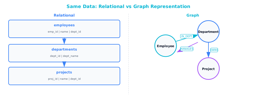 If you have spent your career in the relational world, you have a deeply ingrained mental model for how data is stored. Tables have rows, rows have columns, and tables are connected through foreign keys. Queries use JOINs to follow those foreign keys and combine data from multiple tables.
Graph databases use different vocabulary for the same fundamental concepts, and the fastest way to learn is to map one vocabulary to the other.
| Relational Concept | Graph Concept | What It Means |
|---|---|---|
| Table | Label (Node type) | A category of things (e.g., Employee, Department) |
| Row | Node | A single entity (e.g., employee #4521) |
| Column | Property | An attribute of that entity (e.g., name, hire_date) |
| Foreign key | Relationship | A connection between two entities |
| JOIN | Traversal | Following a connection to reach related data |
| Junction table (many-to-many) | Relationship with properties | A direct connection that carries its own data |
| Schema (DDL) | Flexible (optional schema) | Graph databases are typically schema-optional |
Think of it like this: In a relational database, relationships are implied by matching values in columns. In a graph database, relationships are physical things. They exist as first-class objects, just like the data they connect. It is the difference between knowing that two people share a phone number (you have to look it up) and seeing them holding the same piece of string (the connection is visible and direct).
02. The Property Graph Model, Explained via HR Data
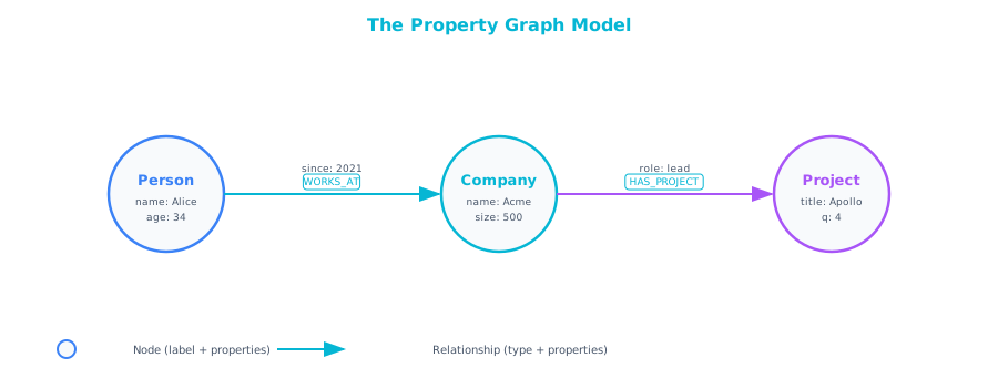
The most common graph model, used by Neo4j, FalkorDB, and most graph databases you will encounter, is the property graph model. It has exactly three building blocks:
- Nodes: the things (entities)
- Relationships: the connections between things (always directed, always have a type)
- Properties: key-value pairs attached to either nodes or relationships
Let us take an HR database you already know and show the same data both ways.
The Relational Version
-- Tables
CREATE TABLE departments (
    dept_id INT PRIMARY KEY,
    name VARCHAR(100),
    location VARCHAR(100)
);

CREATE TABLE employees (
    emp_id INT PRIMARY KEY,
    name VARCHAR(100),
    title VARCHAR(100),
    hire_date DATE,
    salary DECIMAL(10,2),
    dept_id INT REFERENCES departments(dept_id),
    manager_id INT REFERENCES employees(emp_id)
);

CREATE TABLE projects (
    project_id INT PRIMARY KEY,
    name VARCHAR(200),
    status VARCHAR(20),
    budget DECIMAL(12,2)
);

CREATE TABLE employee_projects (
    emp_id INT REFERENCES employees(emp_id),
    project_id INT REFERENCES projects(project_id),
    role VARCHAR(50),
    assigned_date DATE,
    PRIMARY KEY (emp_id, project_id)
);

-- Sample data
INSERT INTO departments VALUES (1, 'Engineering', 'Building A');
INSERT INTO departments VALUES (2, 'Product', 'Building B');

INSERT INTO employees VALUES (101, 'Alice Chen', 'VP Engineering', '2019-03-15', 195000, 1, NULL);
INSERT INTO employees VALUES (102, 'Bob Park', 'Senior Developer', '2020-06-01', 145000, 1, 101);
INSERT INTO employees VALUES (103, 'Carol Reyes', 'Product Manager', '2021-01-10', 135000, 2, NULL);

INSERT INTO projects VALUES (201, 'Data Platform', 'Active', 500000);

INSERT INTO employee_projects VALUES (102, 201, 'Tech Lead', '2024-01-15');
INSERT INTO employee_projects VALUES (103, 201, 'Product Owner', '2024-01-15');
The Graph Version
// Nodes (equivalent to rows)
CREATE (eng:Department {name: 'Engineering', location: 'Building A'})
CREATE (prod:Department {name: 'Product', location: 'Building B'})

CREATE (alice:Employee {name: 'Alice Chen', title: 'VP Engineering',
                        hire_date: date('2019-03-15'), salary: 195000})
CREATE (bob:Employee {name: 'Bob Park', title: 'Senior Developer',
                      hire_date: date('2020-06-01'), salary: 145000})
CREATE (carol:Employee {name: 'Carol Reyes', title: 'Product Manager',
                        hire_date: date('2021-01-10'), salary: 135000})

CREATE (dp:Project {name: 'Data Platform', status: 'Active', budget: 500000})

// Relationships (equivalent to foreign keys and junction table rows)
CREATE (alice)-[:BELONGS_TO]->(eng)
CREATE (bob)-[:BELONGS_TO]->(eng)
CREATE (carol)-[:BELONGS_TO]->(prod)

CREATE (bob)-[:REPORTS_TO]->(alice)

// Notice: the junction table becomes a relationship WITH properties
CREATE (bob)-[:WORKS_ON {role: 'Tech Lead', assigned_date: date('2024-01-15')}]->(dp)
CREATE (carol)-[:WORKS_ON {role: 'Product Owner', assigned_date: date('2024-01-15')}]->(dp)
What Changed
Three things happened in the translation:
-
The
departments,employees, andprojectstables became nodes with labels (Department,Employee,Project). Each row became a node. Each column became a property on that node. -
The foreign keys became relationships. The
dept_idcolumn in the employees table was replaced by aBELONGS_TOrelationship. Themanager_idself-referencing foreign key became aREPORTS_TOrelationship. Foreign keys disappear entirely. They are not needed when the relationship is stored directly. -
The junction table disappeared. The
employee_projectstable, which existed only to connect employees to projects, became aWORKS_ONrelationship with theroleandassigned_datestored as properties on the relationship itself.
Think of it like this: In the relational model, you describe connections with data ("Bob's manager_id is 101, and 101 maps to Alice"). In the graph model, you describe connections with structure ("Bob REPORTS_TO Alice"). The information is identical, but the storage is different. That storage difference is what makes traversal fast.
03. Side-by-Side: The Same Query Both Ways
Let us run a few queries against this HR data to see how the relational and graph approaches differ in practice.
Query 1: Find Bob's manager
SQL:
SELECT m.name AS manager_name
FROM employees e
JOIN employees m ON e.manager_id = m.emp_id
WHERE e.name = 'Bob Park';
Cypher:
MATCH (bob:Employee {name: 'Bob Park'})-[:REPORTS_TO]->(manager)
RETURN manager.name;
Both return "Alice Chen." The Cypher version reads like a sentence: "Find the employee named Bob Park, follow his REPORTS_TO relationship, return the manager's name."
Query 2: Find all employees working on the same project as Bob
SQL:
SELECT DISTINCT e2.name, ep2.role
FROM employees e1
JOIN employee_projects ep1 ON e1.emp_id = ep1.emp_id
JOIN employee_projects ep2 ON ep1.project_id = ep2.project_id
JOIN employees e2 ON ep2.emp_id = e2.emp_id
WHERE e1.name = 'Bob Park'
  AND e2.name != 'Bob Park';
Cypher:
MATCH (bob:Employee {name: 'Bob Park'})-[:WORKS_ON]->(project)<-[w:WORKS_ON]-(colleague)
WHERE colleague <> bob
RETURN colleague.name, w.role;
The SQL requires four JOINs: two passes through the junction table and two through the employees table. The Cypher expresses the pattern directly: Bob works on a project, and someone else also works on that project.
Query 3: Find Bob's manager's other direct reports
SQL:
SELECT e2.name, e2.title
FROM employees e1
JOIN employees m ON e1.manager_id = m.emp_id
JOIN employees e2 ON e2.manager_id = m.emp_id
WHERE e1.name = 'Bob Park'
  AND e2.name != 'Bob Park';
Cypher:
MATCH (bob:Employee {name: 'Bob Park'})-[:REPORTS_TO]->(manager)<-[:REPORTS_TO]-(peer)
WHERE peer <> bob
RETURN peer.name, peer.title;
Again, the Cypher reads like the question: "Start at Bob, go up to his manager, then come back down to anyone else who reports to that manager."
04. How Traversal Actually Works
When the relational database executes a JOIN, it performs a matching operation. It takes a value from one table (say, manager_id = 101) and searches for that value in another table's index. This is a lookup: a search through a data structure.
When a graph database traverses a relationship, it follows a stored pointer. The relationship is not a value to be matched; it is an address to be followed. This is the fundamental mechanism behind the performance characteristics we discussed in Chapter 1.
Here is a step-by-step comparison of what happens when you query "find everyone in Bob's management chain up to the CEO":
Relational Execution (Recursive CTE)
Step 1: Find Bob (index scan on employees.name) → emp_id = 102, manager_id = 101
Step 2: Find manager_id=101 (index scan on employees.emp_id) → Alice, manager_id = NULL
Step 3: manager_id is NULL → stop recursion
Result: [Bob → Alice]
Each step requires an index scan. With a B-tree index on 100,000 employees, each scan examines approximately log2(100,000) = ~17 index nodes. Trivial for two levels, but for a 15-level hierarchy with multiple branches, those scans add up.
Graph Execution (Pointer Traversal)
Step 1: Find Bob (index scan on name property) → node #102
Step 2: Follow REPORTS_TO pointer from node #102 → node #101 (Alice)
Step 3: Node #101 has no outgoing REPORTS_TO → stop
Result: [Bob → Alice]
Step 1 is the same. Both databases need to find the starting node. But Step 2 is different. Instead of searching an index, the graph database reads a pointer from Bob's relationship list. That pointer is a direct memory address (or disk offset) of Alice's node. The cost does not depend on how many employees exist in the database.
Think of it like this: In the relational model, every hop in a traversal is like looking someone up in a phone book. In the graph model, every hop is like already having their phone number in your pocket. The phone book approach works, but it slows down as the phone book gets bigger. The pocket approach takes the same amount of time regardless of how many people exist in the city.
05. Graph Database Comparison: Neo4j, Amazon Neptune, FalkorDB
If you decide a graph database is right for a particular workload, you have several options. Here is a practical comparison of the three you are most likely to evaluate.
| Feature | Neo4j | Amazon Neptune | FalkorDB |
|---|---|---|---|
| Graph model | Property graph | Property graph + RDF | Property graph |
| Query language | Cypher | openCypher, Gremlin, SPARQL | Cypher (subset) |
| Deployment | Self-hosted, Aura (cloud) | AWS managed service | Self-hosted, Cloud |
| Best for | General purpose, most graph workloads | AWS-native teams, RDF requirements | Redis ecosystem, low-latency |
| Strengths | Mature ecosystem, best tooling, largest community | Fully managed, integrates with AWS services | Extremely fast for small-to-medium graphs, Redis compatible |
| Weaknesses | Can be expensive at scale, JVM-based | Vendor lock-in, less community content | Smaller ecosystem, newer |
| Pricing model | Per-node (Aura) or self-hosted | Instance hours + I/O + storage | Open source + commercial support |
| Learning resources | Excellent (GraphAcademy, books, courses) | Good (AWS docs, tutorials) | Growing (docs, community) |
| ACID compliance | Full ACID | Full ACID | Full ACID |
| Maximum graph size | Billions of nodes (Enterprise) | Billions of nodes | Millions of nodes (optimized for speed) |
| Python driver | Official neo4j package | boto3 + gremlinpython | redis + FalkorDB package |
Which One to Choose
For most teams starting with graph databases, Neo4j is the safest choice. It has the largest community, the best learning resources, and the most mature tooling. Its query language (Cypher) is the de facto standard that other databases have adopted (openCypher). If you are already in the AWS ecosystem and want a managed service, Amazon Neptune is a reasonable choice, especially if you have RDF data or need Gremlin compatibility. FalkorDB is compelling if you need very low latency on smaller graphs and are already using Redis.
06. Property Graph vs. RDF: And Why It Matters for AI
You will encounter two fundamentally different graph models in the wild. Understanding the distinction matters, especially as you move toward AI use cases.
Property Graph
This is what we have been discussing. Nodes have labels and properties. Relationships have types and properties. It is intuitive, flexible, and maps well to how most people think about data.
(Alice:Employee {title: "VP"}) -[:MANAGES {since: 2020}]-> (Bob:Employee {title: "Dev"})
RDF (Resource Description Framework)
RDF represents everything as triples: subject-predicate-object. There are no properties on relationships. Everything is a node, and attributes are expressed as relationships to literal values.
<Alice> <rdf:type> <Employee> .
<Alice> <hasTitle> "VP" .
<Alice> <manages> <Bob> .
<Bob> <rdf:type> <Employee> .
<Bob> <hasTitle> "Dev" .
The same data takes more triples to express, and the query language (SPARQL) has a steeper learning curve than Cypher. However, RDF has one significant advantage: it was designed for data interchange and ontology-based reasoning. RDF graphs can link to external knowledge bases (like Wikidata, DBpedia) using standardized URIs, and OWL (Web Ontology Language) allows you to define formal reasoning rules.
Why Property Graphs Win for Most AI Use Cases
| Criterion | Property Graph | RDF |
|---|---|---|
| Ease of learning (for SQL developers) | High | Low |
| Query language familiarity | Cypher (SQL-like) | SPARQL (different paradigm) |
| Performance for traversals | Optimized | Varies |
| Schema flexibility | Schema-optional | Schema-flexible (with ontologies) |
| Integration with LLMs | Strong (LLMs generate Cypher well) | Weaker (SPARQL generation is error-prone) |
| Linking to external knowledge | Manual | Built-in (URI-based) |
| Tooling ecosystem | Large, growing | Established but smaller |
| Best for AI applications | Knowledge graphs, GraphRAG, recommendations | Formal ontologies, linked open data |
Think of it like this: Property graphs are like JSON: flexible, easy to read, and good enough for most applications. RDF is like XML with schemas: more formal, more powerful for interchange, but heavier to work with. If you are building a knowledge graph to power an AI application, start with a property graph. If you are building a standards-compliant knowledge base for a government or academic institution, consider RDF.
For the rest of this book, we will focus on property graphs and Cypher, as they are the most practical path for practitioners coming from the relational world.
07. The Data Model Is the Query
One of the most profound differences between relational and graph databases is this: in a relational database, the data model and the query language are separate concerns. You design your schema (DDL), and then you write queries against it (DML). The schema constrains what you can store, and the query language determines how you retrieve it.
In a graph database, the data model and the query language are nearly the same thing. When you write a Cypher query like:
MATCH (e:Employee)-[:REPORTS_TO]->(m:Employee)-[:BELONGS_TO]->(d:Department)
RETURN e.name, m.name, d.name
The query pattern (e)-[:REPORTS_TO]->(m)-[:BELONGS_TO]->(d) is literally a drawing of the data model. You are describing the shape of the data you want, and the database finds all instances that match that shape.
This has a practical implication: if you can draw the answer on a whiteboard, you can write the query. The Cypher query IS the whiteboard drawing, expressed in text.
Relational queries, by contrast, describe operations (select these columns, join these tables, filter by these conditions). You have to mentally translate between the ERD and the SQL. With Cypher, the translation step disappears.
08. Hands-On: Your First Graph in Python
Let us make this tangible. Here is how to create the HR graph from Section 02 using Python and the Neo4j driver. You can run this against a free Neo4j Aura instance or a local Docker container.
Setting Up
# Install the driver
pip install neo4j

# Or run Neo4j locally with Docker
docker run -d --name neo4j \
  -p 7474:7474 -p 7687:7687 \
  -e NEO4J_AUTH=neo4j/password123 \
  neo4j:5
Creating the Graph
from neo4j import GraphDatabase

# Connect to Neo4j
driver = GraphDatabase.driver("bolt://localhost:7687", auth=("neo4j", "password123"))

def create_hr_graph(tx):
    # Create departments
    tx.run("""
        CREATE (eng:Department {name: 'Engineering', location: 'Building A'})
        CREATE (prod:Department {name: 'Product', location: 'Building B'})

        CREATE (alice:Employee {name: 'Alice Chen', title: 'VP Engineering',
                                hire_date: date('2019-03-15'), salary: 195000})
        CREATE (bob:Employee {name: 'Bob Park', title: 'Senior Developer',
                              hire_date: date('2020-06-01'), salary: 145000})
        CREATE (carol:Employee {name: 'Carol Reyes', title: 'Product Manager',
                                hire_date: date('2021-01-10'), salary: 135000})

        CREATE (dp:Project {name: 'Data Platform', status: 'Active',
                            budget: 500000})

        CREATE (alice)-[:BELONGS_TO]->(eng)
        CREATE (bob)-[:BELONGS_TO]->(eng)
        CREATE (carol)-[:BELONGS_TO]->(prod)

        CREATE (bob)-[:REPORTS_TO]->(alice)

        CREATE (bob)-[:WORKS_ON {role: 'Tech Lead',
                                  assigned_date: date('2024-01-15')}]->(dp)
        CREATE (carol)-[:WORKS_ON {role: 'Product Owner',
                                    assigned_date: date('2024-01-15')}]->(dp)
    """)

with driver.session() as session:
    session.execute_write(create_hr_graph)
    print("HR graph created successfully.")
Querying the Graph
def find_team(tx, project_name):
    result = tx.run("""
        MATCH (e:Employee)-[w:WORKS_ON]->(p:Project {name: $project_name})
        OPTIONAL MATCH (e)-[:REPORTS_TO]->(m:Employee)
        RETURN e.name AS employee, w.role AS role, m.name AS manager
    """, project_name=project_name)
    return [record.data() for record in result]

with driver.session() as session:
    team = session.execute_read(find_team, "Data Platform")
    for member in team:
        print(f"{member['employee']} ({member['role']}) "
              f"- reports to {member['manager'] or 'nobody'}")

# Output:
# Bob Park (Tech Lead) - reports to Alice Chen
# Carol Reyes (Product Owner) - reports to nobody
Querying the Management Chain
def management_chain(tx, employee_name):
    result = tx.run("""
        MATCH (e:Employee {name: $name})-[:REPORTS_TO*1..10]->(m:Employee)
        RETURN m.name AS manager, m.title AS title
        ORDER BY m.salary DESC
    """, name=employee_name)
    return [record.data() for record in result]

with driver.session() as session:
    chain = session.execute_read(management_chain, "Bob Park")
    print(f"Management chain for Bob Park:")
    for manager in chain:
        print(f"  → {manager['manager']} ({manager['title']})")

# Output:
# Management chain for Bob Park:
#   → Alice Chen (VP Engineering)
Notice the REPORTS_TO*1..10 syntax. This tells Neo4j to follow the REPORTS_TO relationship between 1 and 10 hops. If Alice reported to a CTO, and the CTO reported to a CEO, all three would be returned with a single query and no recursive CTE.
09. Mental Model Summary
Here is the mental model that should be forming:
| When you think... | In relational terms... | In graph terms... |
|---|---|---|
| "I need a new type of entity" | Create a table | Create nodes with a new label |
| "I need to connect two entities" | Add a foreign key column | Create a relationship |
| "The connection has its own data" | Create a junction table | Add properties to the relationship |
| "I need to traverse a hierarchy" | Write a recursive CTE | Use variable-length path *1..N |
| "I need to find patterns" | Write complex JOINs with subqueries | Write a MATCH pattern |
| "I need to know all paths between A and B" | Probably give up | Use allShortestPaths() |
10. Chapter Checklist
Before moving on, make sure you can answer these questions:
- Can you explain nodes, relationships, and properties using their relational equivalents?
- Can you look at a simple ERD and sketch the equivalent graph model?
- Do you understand why junction tables disappear in a graph model?
- Can you explain the difference between property graphs and RDF?
- Could you run a simple Cypher query against Neo4j using Python?
If you answered yes to all five, you are ready for Chapter 3, where we connect graph databases to the AI stack and explain why this combination is so powerful.