Chapter 01 of 20
The JOIN Wall
Your compliance query spans 12 tables and takes 4 hours. This chapter explains why deep JOINs hit a performance wall, what graph databases do differently with index-free adjacency, and how to decide whether your workload belongs in a relational database or a graph.
Overview
Your compliance query spans 12 tables and takes 4 hours. Here is why.
01. The Query That Started This Book
 Every organization has one. The query that nobody wants to touch. The stored procedure that a developer wrote three years ago, that everyone is afraid to modify, and that runs during an overnight batch window because it would crush the database during business hours.
Here is a version you will recognize. Your compliance team needs to answer a simple question: "For a given purchase order, show me every person who approved it, their manager chain up to the VP, the vendor that fulfilled it, every subcontractor that vendor used, and every prior audit finding associated with any entity in that chain."
In English, that is one sentence. In SQL, it is a 200-line monster that JOINs 12 tables, uses three CTEs, two subqueries, and a recursive common table expression for the org hierarchy. It works. It returns correct results. And it takes four hours to run against production data.
This chapter is about understanding why that happens, what the actual bottleneck is, and what you should do about it.
02. Why Three-Way JOINs Are Fine but Seven-Way JOINs Kill Performance
If you have spent any time writing SQL, you have an intuitive sense that adding JOINs makes queries slower. The relationship between JOIN depth and performance is not linear. It is closer to exponential, and understanding why requires looking at what the database engine is actually doing.
When you write a two-table JOIN, the query planner picks a strategy: nested loop, hash join, or merge join. For most well-indexed tables, this is fast. The planner has good statistics, the indexes are useful, and the result set is manageable.
When you add a third table, the planner now has to decide the order in which to join all three. There are 3! = 6 possible join orders. The planner evaluates them (or a subset of them), picks the best one, and executes. Still manageable.
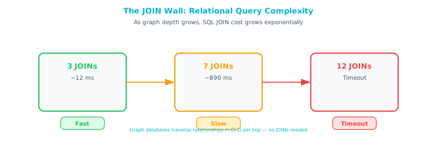
At seven tables, there are 7! = 5,040 possible join orders. At twelve tables, there are 479,001,600. The query planner cannot evaluate all of them, so it uses heuristics. Those heuristics can be wrong. A suboptimal join order on a 12-table query does not make the query 10% slower. It can make it 100x slower.
Think of it like this: Imagine you need to visit 12 offices in a building to collect signatures. If you plan the optimal route, it takes 30 minutes. If you visit them in a random order, backtracking through hallways and waiting for elevators, it takes all day. The database query planner is trying to find the optimal route through your tables, but with 12 stops, it is guessing.
Here is what happens at each stage:
| JOIN Depth | Possible Orders | Planner Behavior | Typical Impact |
|---|---|---|---|
| 2-3 tables | 6 | Evaluates all options | Negligible overhead |
| 4-5 tables | 24-120 | Evaluates most options | Minor overhead |
| 6-7 tables | 720-5,040 | Starts using heuristics | Noticeable slowdown |
| 8-10 tables | 40K-3.6M | Heavy heuristic reliance | Significant risk of bad plans |
| 11-12 tables | 39M-479M | Best-effort estimation | Query plan roulette |
Join order is only half the problem. The other half is the intermediate result set. Each JOIN produces a temporary result that feeds into the next JOIN. If your first JOIN produces 50,000 rows, and the next fans that out to 500,000 rows, and the next fans it to 5 million, you are building a pyramid of temporary data that has to be held in memory or spilled to disk. This is the JOIN wall: the point at which adding one more JOIN does not add a proportional amount of work but multiplies the existing work.
03. A Real Scenario: Tracing an Approval Chain
Let us make this concrete. You have a typical enterprise database with these tables:
-- Simplified schema for an approval/procurement system
CREATE TABLE employees (
    employee_id INT PRIMARY KEY,
    name VARCHAR(100),
    manager_id INT REFERENCES employees(employee_id),
    department_id INT
);

CREATE TABLE purchase_orders (
    po_id INT PRIMARY KEY,
    description VARCHAR(500),
    amount DECIMAL(12,2),
    created_by INT REFERENCES employees(employee_id),
    vendor_id INT
);

CREATE TABLE approvals (
    approval_id INT PRIMARY KEY,
    po_id INT REFERENCES purchase_orders(po_id),
    approver_id INT REFERENCES employees(employee_id),
    approved_at TIMESTAMP,
    decision VARCHAR(20)
);

CREATE TABLE vendors (
    vendor_id INT PRIMARY KEY,
    name VARCHAR(200),
    risk_rating VARCHAR(10)
);

CREATE TABLE vendor_subcontractors (
    vendor_id INT REFERENCES vendors(vendor_id),
    subcontractor_id INT REFERENCES vendors(vendor_id),
    effective_date DATE
);

CREATE TABLE audit_findings (
    finding_id INT PRIMARY KEY,
    entity_type VARCHAR(50),
    entity_id INT,
    finding_text TEXT,
    severity VARCHAR(20),
    found_date DATE
);
The compliance question is: "For PO #4521, show the full approval chain, each approver's management chain up to the VP, the vendor, all subcontractors, and any audit findings on any of these entities."
Here is the SQL:
WITH RECURSIVE manager_chain AS (
    -- Base case: the approvers themselves
    SELECT e.employee_id, e.name, e.manager_id, 1 AS depth
    FROM employees e
    INNER JOIN approvals a ON e.employee_id = a.approver_id
    WHERE a.po_id = 4521

    UNION ALL

    -- Recursive case: walk up the management chain
    SELECT e.employee_id, e.name, e.manager_id, mc.depth + 1
    FROM employees e
    INNER JOIN manager_chain mc ON e.employee_id = mc.manager_id
    WHERE mc.depth < 10  -- safety limit
),
po_vendor AS (
    SELECT po.po_id, po.description, po.amount, v.vendor_id,
           v.name AS vendor_name, v.risk_rating
    FROM purchase_orders po
    INNER JOIN vendors v ON po.vendor_id = v.vendor_id
    WHERE po.po_id = 4521
),
subcontractors AS (
    SELECT vs.vendor_id, vs.subcontractor_id,
           v.name AS sub_name, v.risk_rating AS sub_risk
    FROM vendor_subcontractors vs
    INNER JOIN vendors v ON vs.subcontractor_id = v.vendor_id
    INNER JOIN po_vendor pv ON vs.vendor_id = pv.vendor_id
),
all_entity_ids AS (
    SELECT employee_id AS entity_id, 'employee' AS entity_type
    FROM manager_chain
    UNION ALL
    SELECT vendor_id, 'vendor' FROM po_vendor
    UNION ALL
    SELECT subcontractor_id, 'vendor' FROM subcontractors
)
SELECT
    mc.name AS person,
    mc.depth AS chain_depth,
    pv.vendor_name,
    pv.risk_rating,
    s.sub_name,
    af.finding_text,
    af.severity
FROM manager_chain mc
CROSS JOIN po_vendor pv
LEFT JOIN subcontractors s ON 1=1
LEFT JOIN all_entity_ids aei ON 1=1
LEFT JOIN audit_findings af
    ON af.entity_type = aei.entity_type
    AND af.entity_id = aei.entity_id
ORDER BY mc.depth, s.sub_name, af.severity;
This query is not wrong. It does what was asked. But it has several structural problems that compound as data grows.
04. The Query That Dies at Scale
At 1,000 employees, 500 vendors, and 10,000 purchase orders, this query runs in about 2 seconds. Perfectly acceptable.
At 100,000 employees, 5,000 vendors, and 1,000,000 purchase orders, the same query takes over 4 hours. Here is why:
The recursive CTE is doing full table scans. Each level of the manager chain recursion requires a lookup against the employees table. Without careful indexing, each recursion level scans the entire table. With 10 levels of hierarchy and 100,000 employees, that is up to 1 million row comparisons just for the org chart.
The CROSS JOIN creates a cartesian product. The final SELECT joins the manager chain results with the vendor and subcontractor results, producing a combinatorial explosion. If there are 15 people in the approval/manager chain and 8 subcontractors, that is 120 rows before you even get to audit findings.
The audit findings lookup is a polymorphic query. The entity_type + entity_id pattern (sometimes called a polymorphic association) prevents the database from using foreign key indexes efficiently. It has to scan audit_findings for each combination of entity type and ID.
The query planner gives up on optimization. With recursive CTEs, CROSS JOINs, and polymorphic lookups, the query planner has very little room to optimize. It essentially runs the query in the order you wrote it, which may not be the best order.
Think of it like this: You asked one person to hand-deliver a memo to every office in a 50-story building, wait for a response at each one, and bring all the responses back sorted. At 10 offices, that is an afternoon. At 1,000 offices, that person quits.
Here is a rough timeline of how this query degrades as data grows:
| Data Scale | Employees | Vendors | POs | Approx. Query Time | User Experience |
|---|---|---|---|---|---|
| Small | 1,000 | 500 | 10,000 | 2 seconds | Interactive |
| Medium | 10,000 | 1,000 | 100,000 | 30-90 seconds | User waits, gets coffee |
| Large | 100,000 | 5,000 | 1,000,000 | 15-60 minutes | Batch job territory |
| Enterprise | 500,000 | 20,000 | 10,000,000 | 2-8 hours | Overnight process |
The data grew by 500x (from 1,000 to 500,000 employees) but the query time grew by roughly 10,000x (from 2 seconds to 4+ hours). That is the JOIN wall. The cost is not proportional to the data. It is proportional to the number of relationships that need to be computed at query time multiplied by the depth of those relationships.
05. What Graph Databases Do Differently
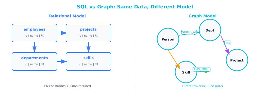
A graph database stores relationships as physical connections between records, not as values in a column that need to be matched at query time. This is the single most important concept in this book. It is called index-free adjacency.
In a relational database, when you write JOIN employees e ON e.employee_id = mc.manager_id, the database has to:
- Take the
manager_idvalue from the current row - Look it up in an index on the
employeestable - Follow that index to the physical row location
- Read the row
That index lookup has a cost, and it is proportional to the size of the index (typically O(log n) for a B-tree). As your employees table grows from 1,000 to 1,000,000 rows, each lookup gets slower. The degradation is not dramatic, but it is consistent.
In a graph database, the relationship between an employee and their manager is stored as a direct pointer. When you traverse from an employee to their manager, the database follows that pointer directly to the manager record. There is no index lookup and no table scan. The cost of that traversal is O(1): constant time, regardless of how many employees exist in the database.
Relational (each hop requires an index lookup):
Employee #7432 → lookup manager_id=2198 in index → scan to row → Employee #2198

Graph (each hop follows a direct pointer):
Employee #7432 → [REPORTS_TO] → Employee #2198
For a single lookup, the difference is negligible. For a 10-level traversal across 100,000 records, it is the difference between seconds and hours.
To understand why the difference compounds, consider what happens when you traverse a 10-level management chain in each model:
Relational (recursive CTE):
- Find the starting employee (index lookup: log2(n) comparisons)
- Find their manager (index lookup: log2(n) comparisons)
- Find that manager's manager (index lookup: log2(n) comparisons)
- ... repeat for each level ...
- Total: 10 x log2(n) index node comparisons
With 1,000,000 employees, that is 10 x 20 = 200 index node comparisons. That sounds fast, but each comparison involves disk I/O or cache lookups, and the recursive CTE machinery adds overhead for materializing intermediate results, checking termination conditions, and deduplicating rows at each level.
Graph (pointer traversal):
- Find the starting employee (index lookup, same as relational; you pay this once)
- Read the REPORTS_TO pointer (one memory read: O(1))
- Follow the pointer to the manager node (one memory read: O(1))
- ... repeat for each level ...
- Total: 1 index lookup + 10 pointer follows
The graph pays the same index cost once to find the starting node, then follows 10 pointers. Each pointer follow is a constant-time operation. It does not depend on how many nodes exist in the database. This is why graph databases maintain their performance as data grows, while relational queries degrade.
Think of it like this: In a relational database, every hop in a hierarchy is like looking up a name in a phone book. The phone book works, but it gets slower as more names are added. In a graph database, every hop is like following a hyperlink on a web page. You click and you are there, regardless of how many pages exist on the internet.
Here is the same compliance query expressed in Cypher, the query language for Neo4j:
// Find PO, its approval chain, manager hierarchies,
// vendor, subcontractors, and audit findings
MATCH (po:PurchaseOrder {po_id: 4521})<-[:APPROVED]-(approver:Employee)
MATCH (approver)-[:REPORTS_TO*1..10]->(manager:Employee)
MATCH (po)-[:FULFILLED_BY]->(vendor:Vendor)
OPTIONAL MATCH (vendor)-[:SUBCONTRACTS]->(sub:Vendor)
OPTIONAL MATCH (entity)-[:HAS_FINDING]->(finding:AuditFinding)
WHERE entity IN collect(DISTINCT approver) + collect(DISTINCT manager)
      + [vendor] + collect(DISTINCT sub)
RETURN approver.name, manager.name, vendor.name,
       sub.name, finding.text, finding.severity
This is not just shorter — it is structurally different. The REPORTS_TO*1..10 syntax says "follow the REPORTS_TO relationship up to 10 hops," and the database does not recursively join a table against itself but walks pointers directly. The FULFILLED_BY and SUBCONTRACTS relationships are traversed directly, not computed through key matching.
The performance characteristics are fundamentally different:
| Operation | Relational (1M rows) | Graph (1M nodes) |
|---|---|---|
| Single relationship lookup | ~0.1ms (index) | ~0.01ms (pointer) |
| 10-level hierarchy traversal | ~500ms-5s | ~1-10ms |
| Variable-depth path finding | Recursive CTE, 1-60s | Pattern match, 1-100ms |
| "All paths between A and B" | Often impractical | Built-in function, <1s |
| Full compliance query | 30min-4hrs | 50ms-2s |
06. When Relational Is Still the Right Choice
Before you start re-architecting everything, understand this: relational databases are the right choice for the vast majority of enterprise workloads. Graph databases solve a specific class of problems exceptionally well, but they are not a general-purpose replacement.
Relational databases excel when:
- Your data is tabular by nature. Customer records, invoices, product catalogs, employee profiles: if your data naturally fits into rows and columns with well-defined schemas, a relational database is purpose-built for it.
- Your queries are predictable and shallow. If most of your queries involve 1-3 table JOINs, filtering, and aggregation, the relational model is fast, mature, and well-tooled.
- ACID transactions are critical. Graph databases support transactions, but relational databases have four decades of battle-tested transaction processing. For financial systems, inventory management, and anything where "exactly once" matters, relational is the safe bet.
- Reporting and analytics are primary use cases. SQL's aggregation capabilities (GROUP BY, HAVING, window functions, ROLLUP) are unmatched. Graph query languages have aggregation, but it is not their strength.
- Your team knows SQL. This is not a trivial consideration. The operational cost of running a technology that your team does not know how to debug at 2 AM is real.
Think of it like this: A relational database is a filing cabinet. It is excellent for storing, organizing, and retrieving documents. A graph database is a corkboard with string connecting the pins. It is excellent for seeing how things connect to each other. You would not replace your filing cabinet with a corkboard, and you would not replace your corkboard with a filing cabinet. You would use both.
07. Decision Table: Relational vs. Graph by Use Case
Use this table when someone asks "should we use a graph database for this?" The answer is almost never "replace your relational database." It is usually "add a graph database for the workloads where relationships are the primary concern."
| Use Case | Relational | Graph | Why |
|---|---|---|---|
| Customer CRUD (create, read, update, delete) | Best choice | Overkill | Tabular data, simple queries |
| Monthly financial reporting | Best choice | Poor fit | Aggregation-heavy, SQL excels |
| Org chart traversal (who reports to whom, 10 levels deep) | Painful | Best choice | Variable-depth hierarchy |
| Fraud detection (find rings of related transactions) | Very difficult | Best choice | Pattern matching across networks |
| Product catalog | Best choice | Possible | Tabular with simple categories |
| Product recommendations ("people who bought X also bought Y") | Difficult at scale | Best choice | Relationship traversal |
| Approval chain tracing | Painful | Best choice | Multi-hop path queries |
| Simple e-commerce transactions | Best choice | Overkill | ACID, tabular, well-understood |
| Supply chain dependency mapping | Difficult | Best choice | Deep, variable-length chains |
| Knowledge management for AI | Poor fit | Best choice | Interconnected concepts, semantic relationships |
| Time-series data (IoT sensors, logs) | Specialized DB | Poor fit | Neither is ideal; use a time-series DB |
| User session tracking | Best choice | Overkill | Simple inserts and lookups |
| Impact analysis (if system X fails, what is affected?) | Very difficult | Best choice | Cascading relationship traversal |
| Compliance audit trails | Painful | Best choice | Multi-entity, multi-hop tracing |
The pattern should be clear: if your query primarily asks "what are the attributes of this entity?" relational wins. If your query primarily asks "how is this entity connected to other entities, and what does the path between them look like?" graph wins.
08. What the EXPLAIN Plan Tells You
If you have access to your database's query plan (EXPLAIN ANALYZE in PostgreSQL, execution plans in SQL Server, or EXPLAIN in MySQL), you can see the JOIN wall forming before it crashes your production database. Here is what to look for.
Signs You Are Hitting the JOIN Wall
Nested Loop Joins on large tables. When you see the planner choosing nested loop joins for tables with more than 10,000 rows, it often means there is no better strategy available. Each nested loop multiplies the rows by the inner table's matching rows.
→  Nested Loop  (cost=0.43..124856.32 rows=5043200 width=128)
     →  Nested Loop  (cost=0.29..48923.15 rows=50432 width=96)
          →  Seq Scan on audit_findings  (rows=12608)
Sequential scans in recursive CTEs. Recursive CTEs often cannot use indexes efficiently because the recursive term generates new rows that need to be looked up in the next iteration. If your EXPLAIN shows sequential scans inside a CTE, the recursion is scanning the full table on each pass.
High estimated row counts between joins. If the planner estimates 50,000 rows coming out of one join and feeding into the next, and that next join is a nested loop, you are about to compute 50,000 x N comparisons. Watch for these intermediate row counts ballooning.
Disk-based sorts and hash tables. When intermediate results are too large for memory, the database spills them to disk. Look for "Sort Method: external merge" or "Hash Batch" counts greater than 1 in PostgreSQL, or "TempDB usage" in SQL Server.
What You Can Do in SQL (Before Adding a Graph)
Before introducing a new technology, you should try optimizing within the relational model. Sometimes the JOIN wall can be pushed back:
| Optimization | What It Does | Limitation |
|---|---|---|
| Add composite indexes | Speeds up specific JOIN conditions | Does not help with variable-depth traversal |
| Materialize CTEs | Pre-computes recursive results | Stale data, maintenance overhead |
| Denormalize tables | Eliminates JOINs by pre-joining data | Data redundancy, update anomalies |
| Partition large tables | Reduces scan range for each JOIN | Only helps if partitions align with queries |
| Increase work_mem / sort_buffer | Keeps intermediate results in memory | Does not reduce computational complexity |
| Limit recursion depth | Prevents runaway recursive CTEs | Silently drops deep relationships |
If you have tried these and the query is still too slow, or if the optimization makes the schema too complex to maintain, that is when a graph database enters the conversation.
09. The Cost of Not Choosing (And the Workarounds That Hide It)
The most common mistake is not choosing at all. Teams hit the JOIN wall, recognize the problem, and then do one of three things:
-
Denormalize the relational schema. They flatten the hierarchy into a single wide table, pre-computing relationships. This works but creates a maintenance burden: every time the org chart changes, the denormalized table needs to be rebuilt.
-
Cache the results. They run the expensive query overnight and cache the results. This works for reporting but cannot handle ad-hoc queries. When the compliance team asks a slightly different question, someone has to modify the batch job and wait until tomorrow.
-
Accept the slowness. They tell users "that report takes 4 hours" and everyone works around it. This is the most common approach and the most insidious. It changes how people use data. They stop asking questions because the answers take too long.
All three of these are signs that your data has outgrown the relational model for this specific workload. Not for all workloads. For this one.
10. What Comes Next
The rest of this book is structured around a practical migration path. You do not need to abandon your relational databases. You do not need to learn an entirely new way of thinking about data. You need to learn which parts of your data model are hitting the JOIN wall, how to move those parts into a graph, and how to connect the graph to your existing systems. As we will see in Chapter 3, your AI systems have an enormous appetite for connected data.
In the next chapter, we will look at how graph databases actually store and retrieve data, explained in terms of the relational concepts you already know. Nodes are rows, relationships are pre-computed JOINs, and properties are columns. Once you see the mapping, the learning curve flattens considerably.
11. Chapter Checklist
Before moving on, make sure you can answer these questions:
- Can you explain why a 3-table JOIN performs differently than a 12-table JOIN, beyond "more tables = slower"?
- Can you describe index-free adjacency in one sentence?
- Can you identify at least two workloads in your current environment that involve deep, variable-length JOINs?
- Can you articulate when a relational database is still the right choice?
- Do you know the difference between "replace your database" and "add a graph for specific workloads"?
If you answered yes to all five, you are ready for Chapter 2.